How to Find a Linear Regression Equation from a Table: A Step-by-Step Guide

Introduction

In a world increasingly driven by data, the ability to understand and apply linear regression is a game-changer for organizations seeking to enhance their operational efficiency. This powerful statistical technique not only illuminates the relationships between variables but also equips teams with the insights necessary for informed decision-making. As businesses navigate the complexities of data analysis, the integration of linear regression with innovative solutions like Robotic Process Automation (RPA) can streamline workflows, reduce errors, and ultimately foster a culture of data-driven success.

This article delves into the foundations of linear regression, offering a comprehensive guide to its application, interpretation, and the tools available to harness its full potential. By mastering these concepts, organizations can unlock the transformative power of data, paving the way for strategic advancements in their operations.

Understanding Linear Regression: A Foundation

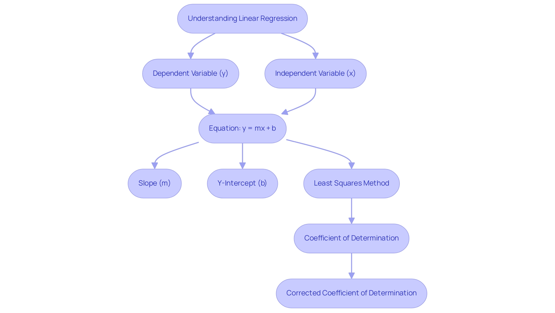
Linear analysis serves as a powerful statistical method for modeling the relationship between a dependent variable and one or more independent variables. Its primary objective is to identify the best-fitting straight line that represents the points, which can be subsequently utilized for prediction. The equation of a linear regression line is expressed as follows:

y = mx + b

In this equation:
– ( y ) represents the dependent variable.
– ( m ) denotes the slope of the line, indicating how much ( y ) changes with a unit change in ( x ).
– ( x ) is the independent variable.
– ( b ) symbolizes the y-intercept, the value of ( y ) when ( x ) equals zero.

A comprehensive grasp of these elements is essential for efficient information analysis, particularly as we examine the most recent uses of predictive models in analytics. Additionally, as organizations strive for operational efficiency, leveraging Robotic Process Automation (RPA) can significantly streamline manual workflows, reducing errors and freeing up valuable resources for more strategic tasks. For example, RPA can streamline the process of examining sales information using a straight-line analysis to forecast upcoming sales patterns, enabling teams to make data-informed choices more effectively.

The least squares method is the most commonly utilized estimation technique in linear analysis, focusing on minimizing the differences between observed and predicted values. For example, recent statistics show that the DCP-VD in the parafoveal region produced a standardized coefficient of -0.485, providing valuable insights into the predictive abilities of the framework. Additionally, the coefficient of determination assesses the accuracy of a statistical framework by indicating the proportion of variation in the dependent variable accounted for by the framework.

It is essential to note that this measure can be artificially inflated by including many independent variables, thus the corrected coefficient of determination is recommended for a more accurate assessment. As Jim aptly notes,

If X and M share variance in predicting Y, when both are included, they might ‘compete’ for explaining the variance in Y.
This emphasizes the significance of thoughtfully examining the connections between variables when building statistical models.

Mastery of these fundamentals, combined with RPA strategies, will empower you to not only learn how to find linear regression equation from a table effectively but also harness their potential for impactful decision-making in your operations. In the context of the rapidly evolving AI landscape, organizations face challenges in identifying the right technologies that align with their business goals. By comprehending and utilizing statistical modeling insights through RPA, companies can address these challenges more efficiently.

To continue learning about these concepts and more, users can log in with Google or email for free access to further resources.

Step-by-Step Guide to Finding a Linear Regression Equation

To obtain the regression equation from a table of values, follow these essential steps:

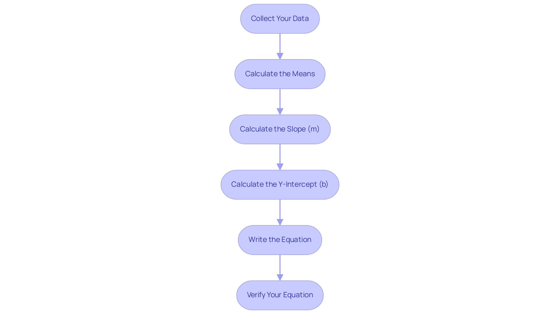
1. Collect Your Data: Begin by ensuring you have a structured table with at least two columns: one representing the independent variable (X) and the other for the dependent variable (Y).

2. Calculate the Means: Compute the mean (average) for both sets of values. The formulas are as follows:

3. Mean of X: \bar{X} = \frac{\sum X}{n}

4. Mean of Y: \bar{Y} = \frac{\sum Y}{n}

5. Calculate the Slope (m): Determine the slope using the formula:
   m = \frac{n(\sum XY) - (\sum X)(\sum Y)}{n(\sum X^2) - (\sum X)^2}
   Here, n denotes the number of data points, \sum XY represents the sum of the products of corresponding X and Y pairs, and \sum X^2 is the sum of the squares of the X values.

6. Calculate the Y-Intercept (b): Next, find the Y-intercept with the formula:
   b = \bar{Y} - m\bar{X}

7. Write the Equation: Substitute the calculated values of m and b into the standard linear equation format:
   y = mx + b

8. Verify Your Equation: Optionally, to ensure accuracy, visualize the points alongside the trend line to confirm the fit. As pointed out by statistician Rebecca Bevans,

   It determines the line of best fit through your data by searching for the value of the coefficient(s) that minimizes the total error of the model.
   This verification step can boost your trust in the outcomes. Furthermore, the results of basic modeling suggest a significant connection between income and happiness. Numerous analyses have indicated significant links between biking, smoking, and heart disease, further showcasing the adaptability of statistical models in diverse situations.

In practice, a prediction calculator employs these models to forecast dependent variables based on independent values, establishing confidence and prediction intervals. For a practical application, examine the case study titled ‘Value Calculation for Test Evaluation,’ which describes the steps to compute the test value using a correlation coefficient and sample size. For instance, for a sample size of 8 and r = 0.454, the straight-line analysis test value T is determined to be roughly 1.24811026.

By following these steps and taking these insights into account, you can effectively learn how to find the linear regression equation from a table, paving the way for deeper analysis in Power BI.

Tools and Software for Linear Regression Analysis

A variety of tools and software can greatly improve your capability to conduct analysis of relationships efficiently:

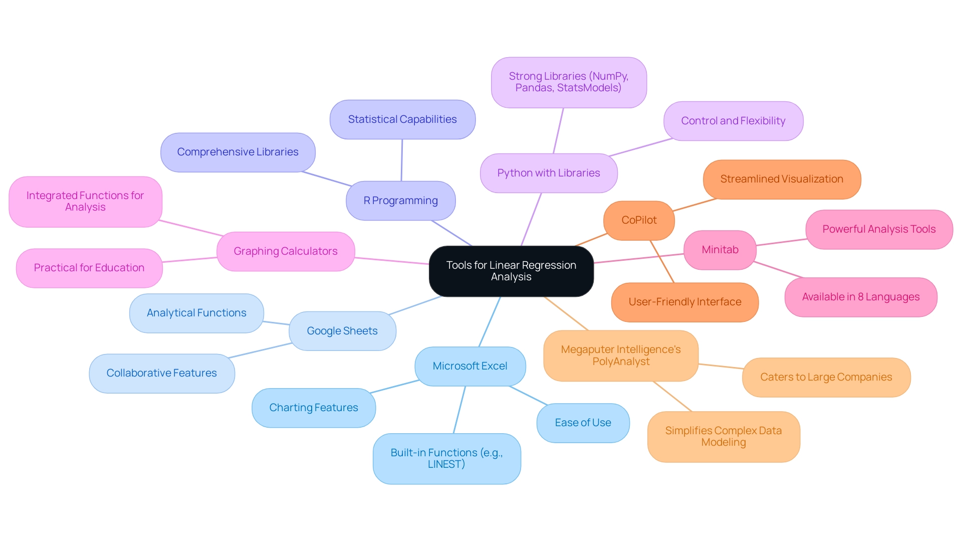
1. Microsoft Excel: This widely accessible tool is favored for its ease of use, allowing for quick calculations through built-in functions like LINEST. Its charting features also facilitate visual representation of trends, making it a preferred choice for many professionals.
2. Google Sheets: Comparable to Excel, Google Sheets offers functions to perform analytical processes and is especially beneficial for collaborative projects, allowing multiple users to examine information at the same time.
3. R Programming: Recognized for its statistical capabilities, R features comprehensive libraries designed for fitting models, making it suitable for managing intricate datasets that necessitate advanced analysis.
4. Python with Libraries (e.g., NumPy, Pandas, StatsModels): As noted by Mark Stent, a Director and Data Scientist,
   

   I am a programmer and like to have a deeper level of control so Python is my go-to tool.
   This programming language offers strong libraries that effectively handle straightforward modeling and information manipulation, attracting individuals with programming skills.

5. Graphing Calculators: Many contemporary graphing calculators feature integrated functions for straight-line analysis, making them a practical option for swift computations, particularly in educational settings.
6. Minitab: Available in 8 languages, Minitab is another powerful tool that supports users from diverse backgrounds, enhancing accessibility for a wider range of analysts.
7. CoPilot: This tool streamlines visualization and analysis with an intuitive interface, making it a superb choice for individuals who value simplicity in conjunction with efficient information representation.

As we look forward to 2024, the environment of software for straight-line analysis continues to develop. Megaputer Intelligence’s PolyAnalyst stands out for its ability to simplify complex data modeling, catering to large companies in need of advanced analytics. Each of these tools has its unique benefits, and the best software ultimately depends on your specific needs and proficiency level.

This is further emphasized in the case study on Intellectual Productivity and Software Choice, which discusses the importance of selecting software that enhances individual productivity, suggesting that the best software choice varies based on user needs and capabilities.

Interpreting the Results of Linear Regression Analysis

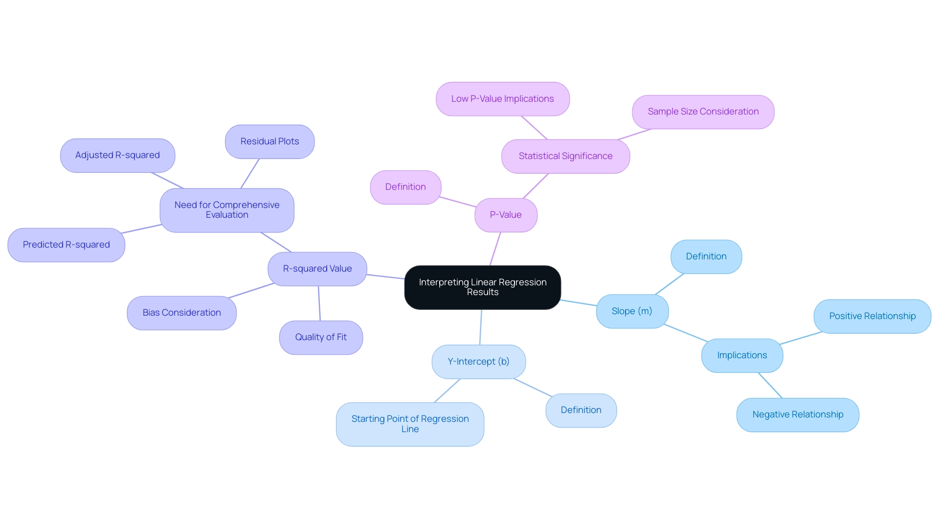
Interpreting the results from your linear analysis equation is a vital step in understanding the relationship between variables within the context of Business Intelligence. Here’s a breakdown of the key components:

1. Slope (m): This value represents the change in the dependent variable (Y) for each unit increase in the independent variable (X). A positive slope indicates a direct relationship, meaning as X increases, Y also increases. Conversely, a negative slope signifies an inverse relationship, where an increase in X results in a decrease in Y.

2. Y-Intercept (b): The y-intercept provides the expected value of Y when X is zero, serving as the starting point of the regression line. Understanding this context aids in interpreting the broader implications of the framework, particularly in overcoming challenges such as poor master data quality.

3. R-squared Value: This statistic measures the proportion of variance in the dependent variable explained by the independent variables, indicating the quality of fit. An R-squared value nearing 1 suggests a strong correlation, while a value closer to 0 reflects a weak relationship. However, it’s crucial to remember that recent findings indicate the R-squared in output results can be a biased estimate of the true population R-squared, underscoring the need for careful evaluation. Moreover, as highlighted in the case study titled “Evaluating R-Squared in Regression Analysis,” R-squared should not be evaluated in isolation; it is important to assess it alongside residual plots and other statistics for a comprehensive understanding of your model’s performance. This method is essential in tackling the time-consuming report creation process that frequently obstructs effective decision-making, especially when organizations face challenges with information extraction.

4. P-Value: This statistic assists in assessing the statistical significance of your results. A low p-value (typically less than 0.05) suggests that the observed relationship is statistically significant. As highlighted by a data analyst, statistical significance (rejecting the null hypothesis of zero coefficients) involves the observed R^2 and the sample size n. This highlights that even small effects can be significant with a sufficiently large sample size, emphasizing the importance of considering both R-squared and sample size in your analysis. The connection between R-squared and sample size is vital for grasping the implications of the p-value in statistical analysis, which is essential for utilizing insights from Power BI dashboards effectively.

Along with these main elements, it is advantageous to assess R-squared with other metrics, like adjusted R-squared and predicted R-squared, to achieve a thorough insight into your model’s performance, as indicated by the case study analyzing R-squared in statistical analysis. This holistic view aids in overcoming barriers to AI adoption and enhances overall operational efficiency. Furthermore, incorporating RPA solutions can significantly improve efficiency and address task repetition fatigue, ultimately helping businesses avoid the competitive disadvantage of lacking actionable insights from their data.

Common Challenges and Considerations in Linear Regression

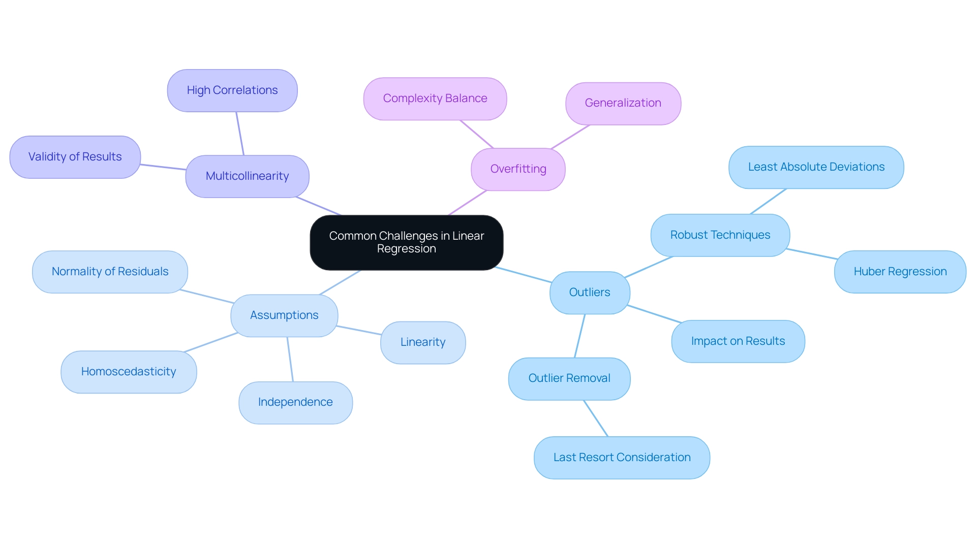
When performing a straight-line analysis, it is essential to identify and tackle various typical issues to improve the dependability of your evaluation:

1. Outliers: Extreme values can significantly skew results, affecting both the slope and intercept of your framework. It’s vital to conduct thorough analyses for outliers, as they can distort your insights. Jose Mendoza emphasizes the significance of this when he observes,
   

   In my work with linear equations, I’ve addressed the issue of outliers by re-estimating analyses after outlier removal and comparing results to comprehend their impact. Additionally, I use robust regression techniques like least absolute deviations and Huber regression, which are less affected by outliers. This proactive approach ensures that the generated systems maintain their reliability. Moreover, it is essential to consider the deletion of outliers as a last resort, given that information is a limited resource and losing it can reduce model performance.

Assumptions of Linear Regression: The validity of your analysis hinges on your data meeting specific assumptions, including linearity, independence, homoscedasticity, and normality of residuals. Violations of these assumptions can lead to misleading conclusions, underscoring the need for rigorous diagnostic checks. Researchers are encouraged to draw scatterplots, calculate least squares lines, and find correlation coefficients to assess how to find linear regression equation from a table in order to determine the appropriateness of linear models.

1. Multicollinearity: In multiple modeling contexts, high correlations among independent variables can distort outcomes. It is critical to check for multicollinearity to ensure the validity of your regression results, thus maintaining the integrity of your analysis.

2. Overfitting: Striking a balance in complexity is essential. An excessively intricate system may perform well with training data but struggle with new data due to overfitting. Aim for a framework that generalizes effectively while still capturing the underlying patterns within the data.

Understanding and addressing these challenges is fundamental to executing a successful linear analysis. Furthermore, consider the findings from recent studies that emphasize the careful handling of outliers as a last resort. The case study on calculating residuals and the Sum of Squared Errors (SSE) illustrates how identifying outliers and evaluating residuals can significantly enhance model performance and accuracy.

For instance, with a maximum age (RIDAGEYR) of 80.0 in your dataset, it is vital to assess how such extreme values may impact your regression analysis, ensuring that your conclusions remain valid and reliable.

Conclusion

The exploration of linear regression reveals its critical role in understanding the relationships between variables, ultimately driving improved decision-making within organizations. By establishing a solid foundation in linear regression principles, teams can effectively model their data, derive meaningful insights, and leverage these findings to enhance operational efficiency.

The step-by-step approach to calculating linear regression equations provides a practical framework for practitioners, empowering them to transform raw data into actionable intelligence. Coupled with the right tools—whether it’s Microsoft Excel, R, or Python—organizations can harness the power of linear regression to analyze trends, predict outcomes, and make informed strategic decisions.

Interpreting the results of linear regression analysis is equally vital. Recognizing the significance of key metrics such as slope, y-intercept, R-squared, and p-values allows teams to gauge the strength and relevance of their models. Addressing common challenges, including outliers and multicollinearity, further enhances the reliability of analyses, ensuring that insights derived from data are both accurate and valuable.

Incorporating linear regression with Robotic Process Automation presents a unique opportunity for organizations to streamline operations and foster a culture of data-driven success. By mastering these concepts, businesses can not only navigate the complexities of data analysis but also position themselves for strategic advancements in an increasingly competitive landscape. The journey towards operational excellence begins with a commitment to understanding and applying the principles of linear regression effectively.

Unlock your organization’s potential—contact us today to learn how our RPA solutions can enhance your data analysis and operational efficiency!